Bootstrap Diagnostics Guide

Introduction

The tsbs package provides a comprehensive diagnostics system for analyzing bootstrap output. When you run tsbs() with return_diagnostics = TRUE, you receive detailed information about:

Block composition: How bootstrap series are constructed from blocks of the original data
Block statistics: Distribution of block lengths and starting positions
Quality metrics: Comparison of original vs. bootstrap series statistics
Method-specific information: Parameters and settings specific to each bootstrap type

This vignette demonstrates how to use these diagnostics to understand and validate your bootstrap analysis.

Quick Start

library(tsbs)

# Generate sample data: AR(1) process
set.seed(42)
n <- 300
x <- arima.sim(n = n, list(ar = 0.7))

# Run bootstrap with diagnostics enabled
result <- tsbs(

x = as.matrix(x),
  block_length = 10,
  bs_type = "moving",
  n_boot = 300,
  num_boots = 100,
  func = mean,
  return_diagnostics = TRUE
)

# View diagnostics summary
summary(result$diagnostics)
#> ========================================
#>   tsbs Bootstrap Diagnostics Summary
#> ========================================
#> 
#> BOOTSTRAP CONFIGURATION:
#>   Bootstrap type: moving 
#>   Original series length: 300 
#>   Number of variables: 1 
#>   Number of replicates: 100 
#>   Generated: 2026-01-31 10:05:43 
#> 
#> CONFIGURATION PARAMETERS:
#>   bs_type: moving
#>   block_type: overlapping
#>   taper_type: NA
#>   tukey_alpha: NA
#>   block_length: 10
#>   n_boot: 300
#>   num_blocks: NULL (auto-computed)
#>   num_boots: 100
#>   p: NULL (auto-computed)
#>   p_method: NA
#>   num_states: NA
#> 
#> BOOTSTRAP SERIES LENGTHS:
#>   Min: 300 
#>   Max: 300 
#>   Mean: 300 
#> 
#> BLOCK LENGTH STATISTICS:
#>   Total blocks sampled: 2993 
#>   Mean block length: 10.02 
#>   SD block length: 0.48 
#>   Min block length: 10 
#>   Max block length: 20 
#>   Median block length: 10 
#>   25th percentile: 10 
#>   75th percentile: 10 
#>   Mean blocks per replicate: 29.93 
#> 
#> ORIGINAL vs BOOTSTRAP STATISTICS:
#> 
#>   MEANS:
#>     Variable 1 :
#>       Original: -0.1558 
#>       Bootstrap avg: -0.1047 
#>       Bootstrap SD: 0.1271 
#>       Bias: 0.0511 
#> 
#>   LAG-1 AUTOCORRELATION:
#>     Variable 1 :
#>       Original: 0.6094 
#>       Bootstrap avg: 0.5377 
#>       Bootstrap SD: 0.0467 
#> 
#> ========================================

The Diagnostics Object

When return_diagnostics = TRUE, the result contains a diagnostics element of class tsbs_diagnostics. This object stores all diagnostic information and supports print(), summary(), and plot() methods.

# Basic info
print(result$diagnostics)
#> tsbs Bootstrap Diagnostics
#>   Type: moving 
#>   Replicates: 100 
#>   Original series: 300 x 1
#> 
#> Use summary() for detailed diagnostics.
#> Use plot() for visualizations.

# Check class
class(result$diagnostics)
#> [1] "tsbs_diagnostics"

# View internal structure
names(result$diagnostics)
#> [1] "meta"            "blocks"          "series_stats"    "original_stats" 
#> [5] "method_specific" "config"

Structure Overview

The diagnostics object contains:

Component	Description
`meta`	Metadata: bootstrap type, dimensions, timestamp
`blocks`	Block composition data for each replicate
`series_stats`	Per-replicate statistics (means, SDs, autocorrelations)
`original_stats`	Reference statistics from original series
`method_specific`	Bootstrap method-specific diagnostics
`config`	Configuration parameters used

Diagnostic Summary

The summary() method provides a comprehensive text report covering all aspects of the bootstrap analysis.

summary(result$diagnostics)
#> ========================================
#>   tsbs Bootstrap Diagnostics Summary
#> ========================================
#> 
#> BOOTSTRAP CONFIGURATION:
#>   Bootstrap type: moving 
#>   Original series length: 300 
#>   Number of variables: 1 
#>   Number of replicates: 100 
#>   Generated: 2026-01-31 10:05:43 
#> 
#> CONFIGURATION PARAMETERS:
#>   bs_type: moving
#>   block_type: overlapping
#>   taper_type: NA
#>   tukey_alpha: NA
#>   block_length: 10
#>   n_boot: 300
#>   num_blocks: NULL (auto-computed)
#>   num_boots: 100
#>   p: NULL (auto-computed)
#>   p_method: NA
#>   num_states: NA
#> 
#> BOOTSTRAP SERIES LENGTHS:
#>   Min: 300 
#>   Max: 300 
#>   Mean: 300 
#> 
#> BLOCK LENGTH STATISTICS:
#>   Total blocks sampled: 2993 
#>   Mean block length: 10.02 
#>   SD block length: 0.48 
#>   Min block length: 10 
#>   Max block length: 20 
#>   Median block length: 10 
#>   25th percentile: 10 
#>   75th percentile: 10 
#>   Mean blocks per replicate: 29.93 
#> 
#> ORIGINAL vs BOOTSTRAP STATISTICS:
#> 
#>   MEANS:
#>     Variable 1 :
#>       Original: -0.1558 
#>       Bootstrap avg: -0.1047 
#>       Bootstrap SD: 0.1271 
#>       Bias: 0.0511 
#> 
#>   LAG-1 AUTOCORRELATION:
#>     Variable 1 :
#>       Original: 0.6094 
#>       Bootstrap avg: 0.5377 
#>       Bootstrap SD: 0.0467 
#> 
#> ========================================

Interpreting the Summary

Bootstrap Configuration: Shows the bootstrap type, series dimensions, and number of replicates.

Configuration Parameters: Lists all parameters used, including auto-computed values.

Bootstrap Series Lengths: For methods that can produce variable-length series, shows the distribution of lengths.

Block Length Statistics: For block-based methods (moving, stationary, HMM, MSVAR), shows:

Total number of blocks sampled across all replicates
Mean, SD, min, max, and median block lengths
Quartiles (25th and 75th percentiles)
Average blocks per replicate

Original vs Bootstrap Statistics: Compares key statistics between the original series and bootstrap replicates:

Means: Original value, bootstrap average, bootstrap SD, and bias
Lag-1 Autocorrelation: How well the bootstrap preserves temporal dependence

Visualizations

The plot() method generates diagnostic visualizations. You can request specific plot types or generate all applicable plots.

Available Plot Types

# All applicable plots
plot(result$diagnostics, type = "all")

# Specific plots
plot(result$diagnostics, type = "block_lengths")
plot(result$diagnostics, type = "start_positions")
plot(result$diagnostics, type = "means_comparison")
plot(result$diagnostics, type = "acf_comparison")
plot(result$diagnostics, type = "length_distribution")

Block Length Distribution

Shows how block lengths are distributed across all bootstrap replicates. For moving block bootstrap, this should be constant; for stationary bootstrap, it follows a geometric distribution.

plot(result$diagnostics, type = "block_lengths")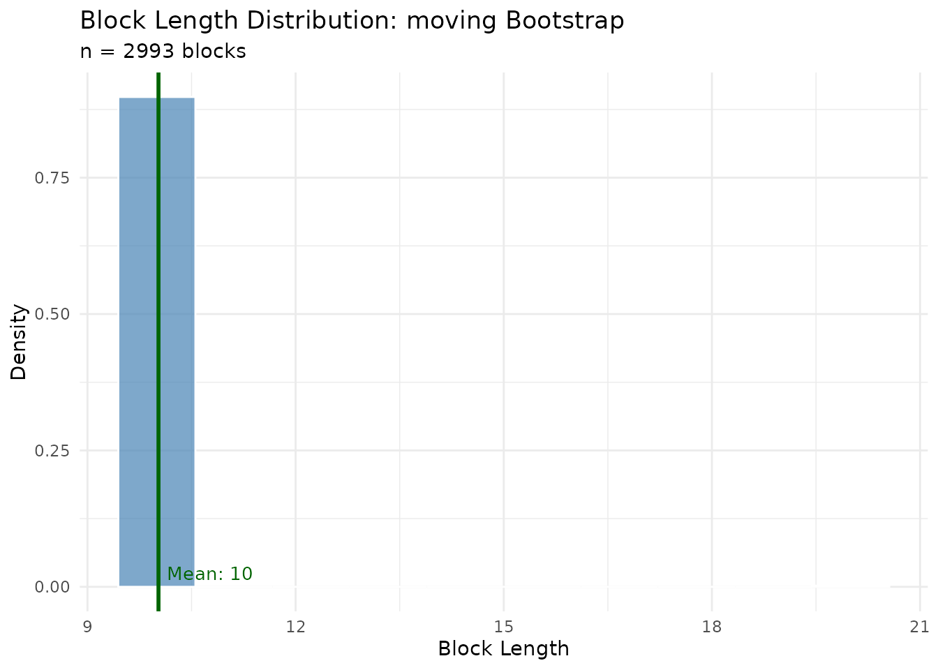

Starting Position Distribution

Shows where blocks are sampled from in the original series. A uniform distribution indicates good coverage of the original data.

plot(result$diagnostics, type = "start_positions")

Means Comparison

Compares the distribution of bootstrap means against the original series mean. The red dashed line shows the original value.

plot(result$diagnostics, type = "means_comparison")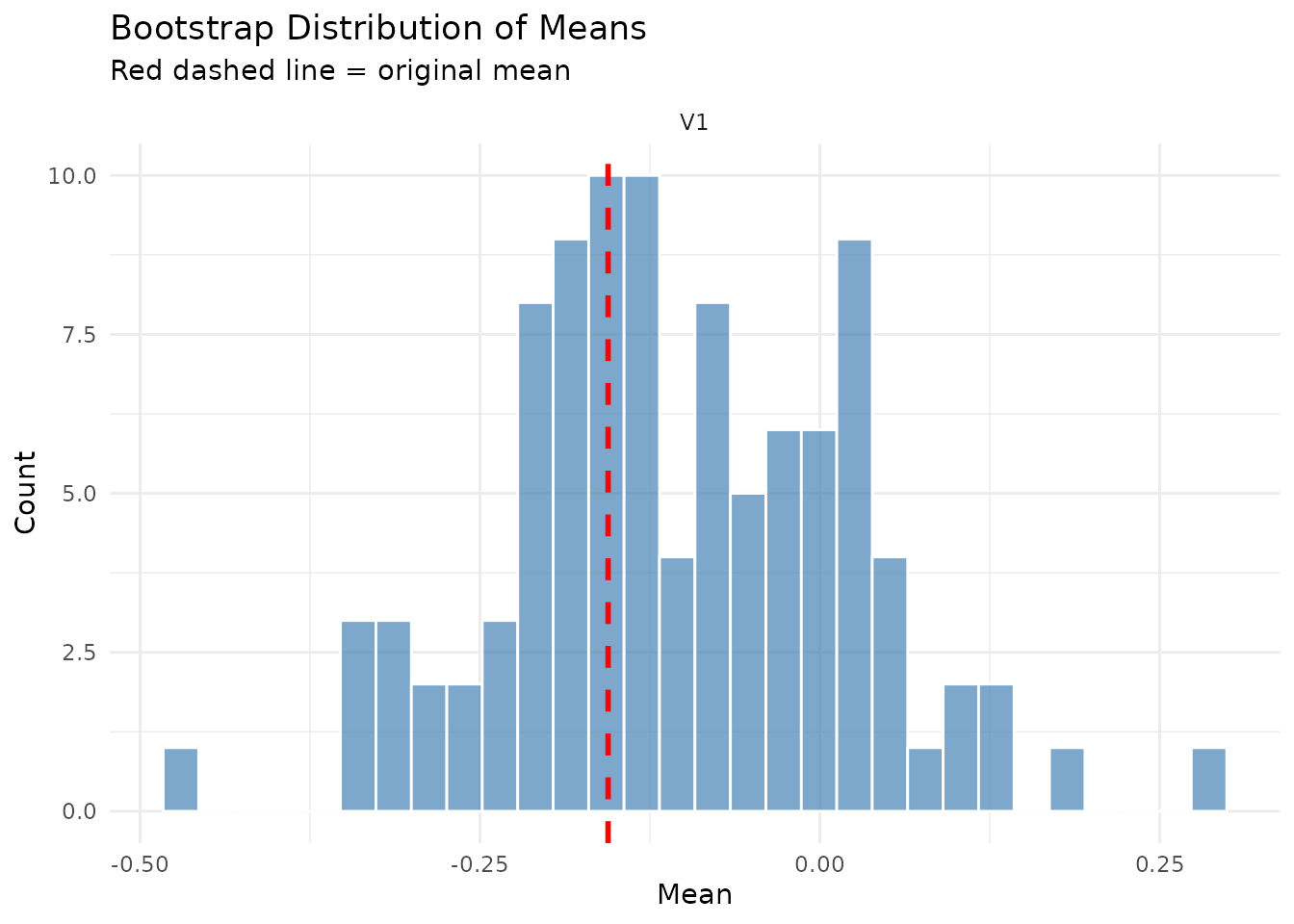

Autocorrelation Comparison

Shows how well the bootstrap preserves the lag-1 autocorrelation structure of the original series.

plot(result$diagnostics, type = "acf_comparison")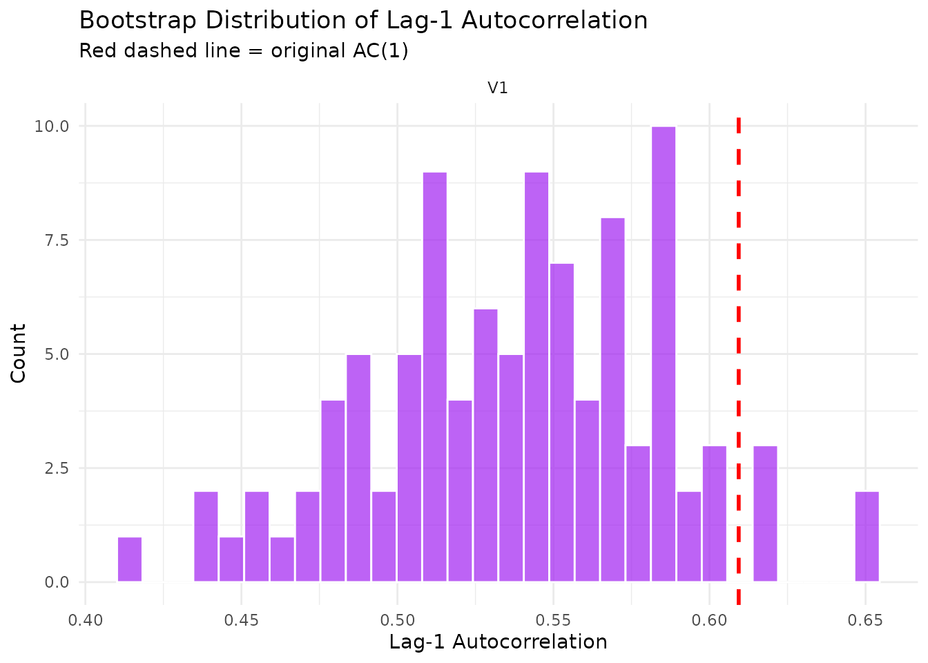

Extracting Diagnostic Data

For custom analysis, you can extract diagnostic data in various formats.

Block Information

# Get all block information
blocks_df <- extract_blocks(result$diagnostics)
head(blocks_df)
#>   block_num length start_pos block_type replicate
#> 1         1     10        32  estimated         1
#> 2         2     10       152  estimated         1
#> 3         3     10       248  estimated         1
#> 4         4     10       208  estimated         1
#> 5         5     10        92  estimated         1
#> 6         6     10        34  estimated         1

# Get blocks for a specific replicate
blocks_rep1 <- extract_blocks(result$diagnostics, replicate = 1)
blocks_rep1
#>    block_num length start_pos block_type
#> 1          1     10        32  estimated
#> 2          2     10       152  estimated
#> 3          3     10       248  estimated
#> 4          4     10       208  estimated
#> 5          5     10        92  estimated
#> 6          6     10        34  estimated
#> 7          7     10       168  estimated
#> 8          8     10       242  estimated
#> 9          9     10       152  estimated
#> 10        10     10       202  estimated
#> 11        11     10       146  estimated
#> 12        12     10       104  estimated
#> 13        13     10       281  estimated
#> 14        14     10       269  estimated
#> 15        15     10        60  estimated
#> 16        16     10       278  estimated
#> 17        17     10       255  estimated
#> 18        18     10       203  estimated
#> 19        19     10       150  estimated
#> 20        20     10       140  estimated
#> 21        21     10        59  estimated
#> 22        22     10        30  estimated
#> 23        23     10       138  estimated
#> 24        24     10        91  estimated
#> 25        25     10       225  estimated
#> 26        26     10       263  estimated
#> 27        27     10        98  estimated
#> 28        28     10       240  estimated
#> 29        29     10        65  estimated
#> 30        30     10       223  estimated

Summary Statistics

# Get comprehensive summary statistics
stats <- extract_summary_stats(result$diagnostics)

# Original series statistics
stats$original
#> $means
#> [1] -0.1558061
#> 
#> $sds
#> [1] 1.218115
#> 
#> $ac1
#> [1] 0.6093509

# Bootstrap statistics with quantiles
stats$bootstrap$means
#> $mean
#> [1] -0.1046991
#> 
#> $sd
#> [1] 0.1271038
#> 
#> $quantiles
#>               [,1]
#> 2.5%  -0.334849152
#> 25%   -0.181688481
#> 50%   -0.120980348
#> 75%   -0.008973198
#> 97.5%  0.119517941

# Block length statistics
stats$block_lengths
#> $mean
#> [1] 10.02339
#> 
#> $sd
#> [1] 0.4831253
#> 
#> $min
#> [1] 10
#> 
#> $max
#> [1] 20
#> 
#> $median
#> [1] 10

Converting to Data Frame

For integration with other analysis workflows, convert diagnostics to a data frame.

# Per-replicate statistics
stats_df <- as.data.frame(result$diagnostics, what = "stats")
head(stats_df)
#>   replicate length       mean_V1    sd_V1    ac1_V1
#> 1         1    300 -0.0004595378 1.170248 0.5127383
#> 2         2    300 -0.0555913842 1.155754 0.5488788
#> 3         3    300 -0.0701734837 1.126817 0.5444252
#> 4         4    300 -0.1803415829 1.204624 0.5368394
#> 5         5    300 -0.0836004992 1.151282 0.4644822
#> 6         6    300  0.2862128585 1.129703 0.4405106

# Block-level data
blocks_df <- as.data.frame(result$diagnostics, what = "blocks")
head(blocks_df)
#>   block_num length start_pos block_type replicate
#> 1         1     10        32  estimated         1
#> 2         2     10       152  estimated         1
#> 3         3     10       248  estimated         1
#> 4         4     10       208  estimated         1
#> 5         5     10        92  estimated         1
#> 6         6     10        34  estimated         1

Bootstrap Type Examples

Different bootstrap methods provide different diagnostic information. This section demonstrates diagnostics for each supported method.

Moving Block Bootstrap

The moving block bootstrap samples fixed-length, overlapping blocks from the original series.

set.seed(123)
x_ar <- as.matrix(arima.sim(n = 200, list(ar = 0.6)))

result_mbb <- tsbs(
  x = x_ar,
  block_length = 12,
  bs_type = "moving",
  block_type = "overlapping",
  n_boot = 200,
  num_boots = 100,
  return_diagnostics = TRUE
)

summary(result_mbb$diagnostics)
#> ========================================
#>   tsbs Bootstrap Diagnostics Summary
#> ========================================
#> 
#> BOOTSTRAP CONFIGURATION:
#>   Bootstrap type: moving 
#>   Original series length: 200 
#>   Number of variables: 1 
#>   Number of replicates: 100 
#>   Generated: 2026-01-31 10:05:45 
#> 
#> CONFIGURATION PARAMETERS:
#>   bs_type: moving
#>   block_type: overlapping
#>   taper_type: NA
#>   tukey_alpha: NA
#>   block_length: 12
#>   n_boot: 200
#>   num_blocks: NULL (auto-computed)
#>   num_boots: 100
#>   p: NULL (auto-computed)
#>   p_method: NA
#>   num_states: NA
#> 
#> BOOTSTRAP SERIES LENGTHS:
#>   Min: 200 
#>   Max: 200 
#>   Mean: 200 
#> 
#> BLOCK LENGTH STATISTICS:
#>   Total blocks sampled: 1688 
#>   Mean block length: 11.85 
#>   SD block length: 1.38 
#>   Min block length: 8 
#>   Max block length: 24 
#>   Median block length: 12 
#>   25th percentile: 12 
#>   75th percentile: 12 
#>   Mean blocks per replicate: 16.88 
#> 
#> ORIGINAL vs BOOTSTRAP STATISTICS:
#> 
#>   MEANS:
#>     Variable 1 :
#>       Original: -0.0018 
#>       Bootstrap avg: -0.0176 
#>       Bootstrap SD: 0.1312 
#>       Bias: -0.0158 
#> 
#>   LAG-1 AUTOCORRELATION:
#>     Variable 1 :
#>       Original: 0.5159 
#>       Bootstrap avg: 0.4697 
#>       Bootstrap SD: 0.061 
#> 
#> ========================================

Key diagnostics for moving block bootstrap:

Block lengths should all equal the specified block_length
Starting positions should be roughly uniformly distributed
Autocorrelation preservation depends on block length relative to data persistence

Stationary Bootstrap

The stationary bootstrap uses geometrically distributed block lengths, providing a stationary resampling scheme.

set.seed(456)

result_sb <- tsbs(
  x = x_ar,
  bs_type = "stationary",
  p_method = "plugin",  # Auto-select p based on autocorrelation
  n_boot = 200,
  num_boots = 100,
  return_diagnostics = TRUE
)

summary(result_sb$diagnostics)
#> ========================================
#>   tsbs Bootstrap Diagnostics Summary
#> ========================================
#> 
#> BOOTSTRAP CONFIGURATION:
#>   Bootstrap type: stationary 
#>   Original series length: 200 
#>   Number of variables: 1 
#>   Number of replicates: 100 
#>   Generated: 2026-01-31 10:05:46 
#> 
#> CONFIGURATION PARAMETERS:
#>   bs_type: stationary
#>   block_type: overlapping
#>   taper_type: NA
#>   tukey_alpha: NA
#>   block_length: NULL (auto-computed)
#>   n_boot: 200
#>   num_blocks: NULL (auto-computed)
#>   num_boots: 100
#>   p: 0.484146996484453
#>   p_method: plugin
#>   num_states: NA
#> 
#> BOOTSTRAP SERIES LENGTHS:
#>   Min: 200 
#>   Max: 200 
#>   Mean: 200 
#> 
#> BLOCK LENGTH STATISTICS:
#>   Total blocks sampled: 9796 
#>   Mean block length: 2.04 
#>   SD block length: 1.38 
#>   Min block length: 1 
#>   Max block length: 11 
#>   Median block length: 2 
#>   25th percentile: 1 
#>   75th percentile: 3 
#>   Mean blocks per replicate: 97.96 
#> 
#> ORIGINAL vs BOOTSTRAP STATISTICS:
#> 
#>   MEANS:
#>     Variable 1 :
#>       Original: -0.0018 
#>       Bootstrap avg: 0.0098 
#>       Bootstrap SD: 0.0901 
#>       Bias: 0.0116 
#> 
#>   LAG-1 AUTOCORRELATION:
#>     Variable 1 :
#>       Original: 0.5159 
#>       Bootstrap avg: 0.2604 
#>       Bootstrap SD: 0.0864 
#> 
#> METHOD-SPECIFIC DIAGNOSTICS:
#>   p_estimated: 0.484146996484453
#>   expected_block_length: 2.06548838939686
#> 
#> ========================================

# Block lengths follow geometric distribution
plot(result_sb$diagnostics, type = "block_lengths")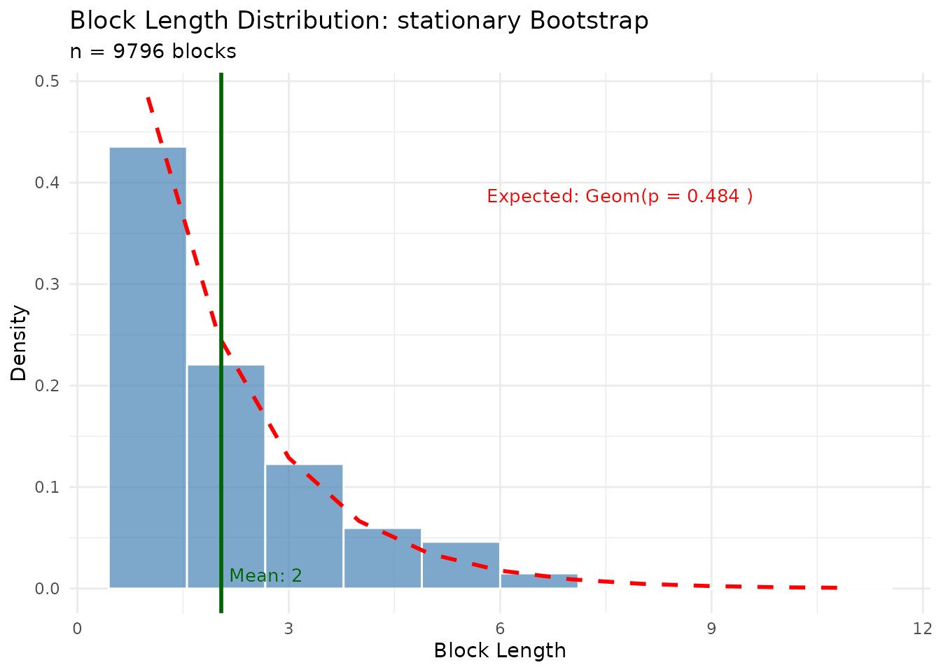

Key diagnostics for stationary bootstrap:

Block lengths follow a geometric distribution
p_estimated shows the geometric parameter used
expected_block_length = 1/p gives the theoretical mean block length
Actual mean block length may differ due to truncation at series boundaries

Tapered Block Bootstrap

Tapered blocks apply window functions to smooth transitions between blocks.

set.seed(789)

result_tapered <- tsbs(
  x = x_ar,
  block_length = 15,
  bs_type = "moving",
  block_type = "tapered",
  taper_type = "tukey",
  tukey_alpha = 0.5,
  n_boot = 200,
  num_boots = 50,
  return_diagnostics = TRUE
)

summary(result_tapered$diagnostics)
#> ========================================
#>   tsbs Bootstrap Diagnostics Summary
#> ========================================
#> 
#> BOOTSTRAP CONFIGURATION:
#>   Bootstrap type: moving 
#>   Original series length: 200 
#>   Number of variables: 1 
#>   Number of replicates: 50 
#>   Generated: 2026-01-31 10:05:47 
#> 
#> CONFIGURATION PARAMETERS:
#>   bs_type: moving
#>   block_type: tapered
#>   taper_type: tukey
#>   tukey_alpha: 0.5
#>   block_length: 15
#>   n_boot: 200
#>   num_blocks: NULL (auto-computed)
#>   num_boots: 50
#>   p: NULL (auto-computed)
#>   p_method: NA
#>   num_states: NA
#> 
#> BOOTSTRAP SERIES LENGTHS:
#>   Min: 200 
#>   Max: 200 
#>   Mean: 200 
#> 
#> BLOCK LENGTH STATISTICS:
#>   Total blocks sampled: 5438 
#>   Mean block length: 1.84 
#>   SD block length: 3.21 
#>   Min block length: 1 
#>   Max block length: 16 
#>   Median block length: 1 
#>   25th percentile: 1 
#>   75th percentile: 1 
#>   Mean blocks per replicate: 108.76 
#> 
#> ORIGINAL vs BOOTSTRAP STATISTICS:
#> 
#>   MEANS:
#>     Variable 1 :
#>       Original: -0.0018 
#>       Bootstrap avg: -0.016 
#>       Bootstrap SD: 0.1457 
#>       Bias: -0.0142 
#> 
#>   LAG-1 AUTOCORRELATION:
#>     Variable 1 :
#>       Original: 0.5159 
#>       Bootstrap avg: 0.4533 
#>       Bootstrap SD: 0.0899 
#> 
#> ========================================

Note: Tapered blocks modify values at block boundaries, which affects the block length estimation heuristic. The estimated block lengths may not perfectly match the actual blocks used.

Wild Bootstrap

The wild bootstrap multiplies observations by random signs (±1), preserving heteroskedasticity patterns. It does not use blocks.

set.seed(321)

# Generate heteroskedastic data
n <- 150
sigma_t <- 1 + 0.5 * sin(2 * pi * (1:n) / 50)
residuals <- as.matrix(rnorm(n) * sigma_t)

result_wild <- tsbs(
  x = residuals,
  bs_type = "wild",
  num_boots = 200,
  return_diagnostics = TRUE
)

summary(result_wild$diagnostics)
#> ========================================
#>   tsbs Bootstrap Diagnostics Summary
#> ========================================
#> 
#> BOOTSTRAP CONFIGURATION:
#>   Bootstrap type: wild 
#>   Original series length: 150 
#>   Number of variables: 1 
#>   Number of replicates: 200 
#>   Generated: 2026-01-31 10:05:48 
#> 
#> CONFIGURATION PARAMETERS:
#>   bs_type: wild
#>   block_type: overlapping
#>   taper_type: NA
#>   tukey_alpha: NA
#>   block_length: NULL (auto-computed)
#>   n_boot: NULL (auto-computed)
#>   num_blocks: NULL (auto-computed)
#>   num_boots: 200
#>   p: NULL (auto-computed)
#>   p_method: NA
#>   num_states: NA
#> 
#> BOOTSTRAP SERIES LENGTHS:
#>   Min: 150 
#>   Max: 150 
#>   Mean: 150 
#> 
#> ORIGINAL vs BOOTSTRAP STATISTICS:
#> 
#>   MEANS:
#>     Variable 1 :
#>       Original: 0.0665 
#>       Bootstrap avg: 0.0024 
#>       Bootstrap SD: 0.0811 
#>       Bias: -0.0641 
#> 
#>   LAG-1 AUTOCORRELATION:
#>     Variable 1 :
#>       Original: -0.0167 
#>       Bootstrap avg: -0.0156 
#>       Bootstrap SD: 0.0919 
#> 
#> ========================================

Key diagnostics for wild bootstrap:

No block statistics (wild bootstrap doesn’t use blocks)
Series length always equals original length
Mean should be approximately zero (signs are randomized)
Variance structure is preserved

plot(result_wild$diagnostics, type = "means_comparison")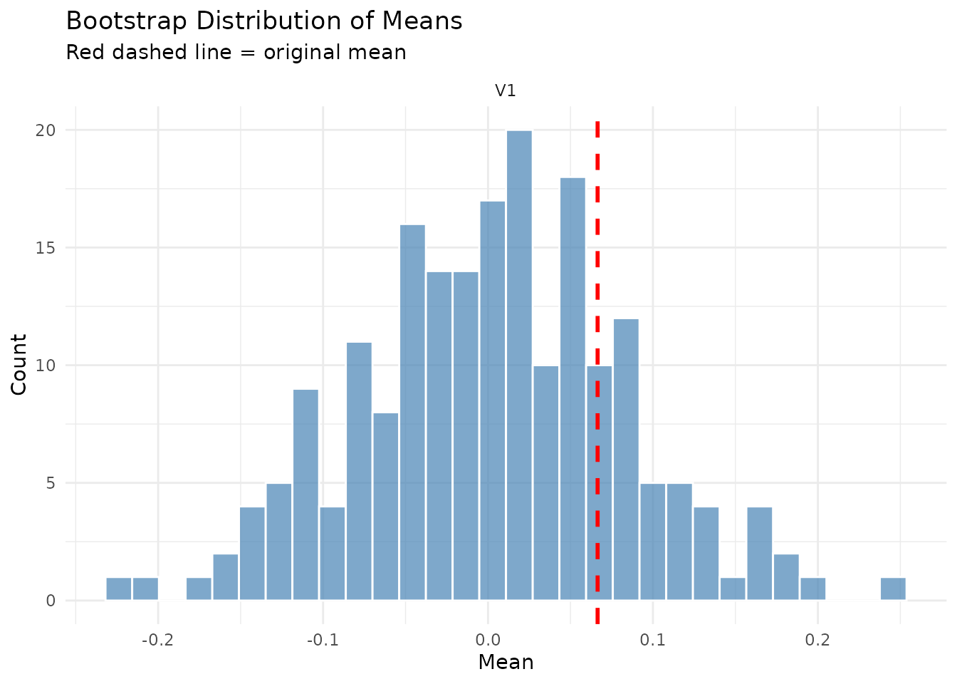

Multivariate Series

The diagnostics system fully supports multivariate time series, providing per-variable statistics.

set.seed(555)

# Generate correlated bivariate series
n <- 200
Sigma <- matrix(c(1, 0.6, 0.6, 1), nrow = 2)
L <- t(chol(Sigma))
innovations <- matrix(rnorm(n * 2), ncol = 2)
x_mv <- innovations %*% t(L)

# Add persistence
for (i in 2:n) {
  x_mv[i, ] <- 0.4 * x_mv[i-1, ] + 0.6 * x_mv[i, ]
}

result_mv <- tsbs(
  x = x_mv,
  block_length = 10,
  bs_type = "moving",
  n_boot = 200,
  num_boots = 100,
  return_diagnostics = TRUE
)

summary(result_mv$diagnostics)
#> ========================================
#>   tsbs Bootstrap Diagnostics Summary
#> ========================================
#> 
#> BOOTSTRAP CONFIGURATION:
#>   Bootstrap type: moving 
#>   Original series length: 200 
#>   Number of variables: 2 
#>   Number of replicates: 100 
#>   Generated: 2026-01-31 10:05:48 
#> 
#> CONFIGURATION PARAMETERS:
#>   bs_type: moving
#>   block_type: overlapping
#>   taper_type: NA
#>   tukey_alpha: NA
#>   block_length: 10
#>   n_boot: 200
#>   num_blocks: NULL (auto-computed)
#>   num_boots: 100
#>   p: NULL (auto-computed)
#>   p_method: NA
#>   num_states: NA
#> 
#> BOOTSTRAP SERIES LENGTHS:
#>   Min: 200 
#>   Max: 200 
#>   Mean: 200 
#> 
#> BLOCK LENGTH STATISTICS:
#>   Total blocks sampled: 1993 
#>   Mean block length: 10.04 
#>   SD block length: 0.59 
#>   Min block length: 10 
#>   Max block length: 20 
#>   Median block length: 10 
#>   25th percentile: 10 
#>   75th percentile: 10 
#>   Mean blocks per replicate: 19.93 
#> 
#> ORIGINAL vs BOOTSTRAP STATISTICS:
#> 
#>   MEANS:
#>     Variable 1 :
#>       Original: 0.0191 
#>       Bootstrap avg: 0.0175 
#>       Bootstrap SD: 0.0449 
#>       Bias: -0.0016 
#>     Variable 2 :
#>       Original: 0.0171 
#>       Bootstrap avg: 0.0259 
#>       Bootstrap SD: 0.0661 
#>       Bias: 0.0088 
#> 
#>   LAG-1 AUTOCORRELATION:
#>     Variable 1 :
#>       Original: 0.3195 
#>       Bootstrap avg: 0.2934 
#>       Bootstrap SD: 0.0634 
#>     Variable 2 :
#>       Original: 0.3538 
#>       Bootstrap avg: 0.2995 
#>       Bootstrap SD: 0.0883 
#> 
#> ========================================

# Means comparison shows both variables
plot(result_mv$diagnostics, type = "means_comparison")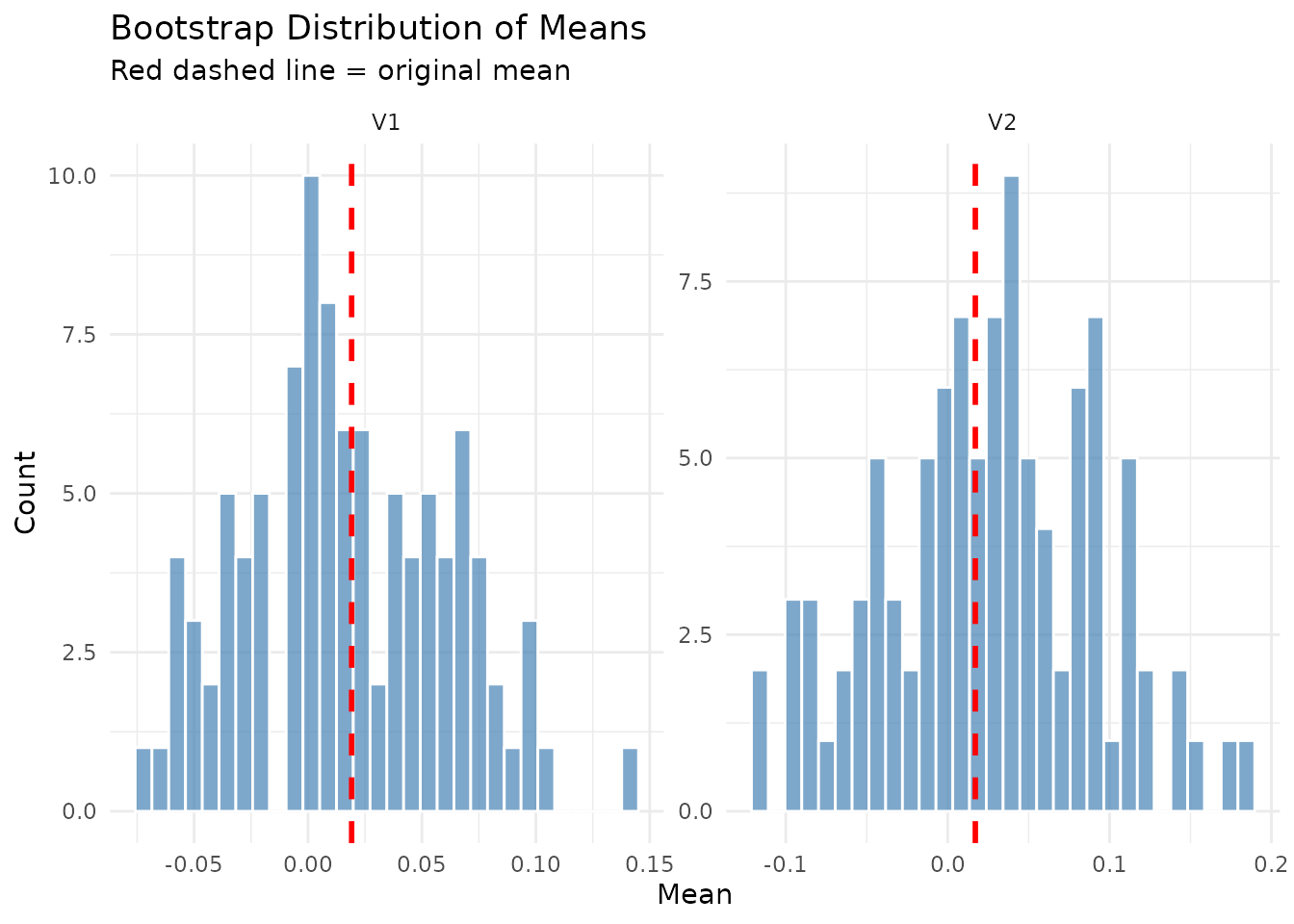


# ACF comparison for each variable
plot(result_mv$diagnostics, type = "acf_comparison")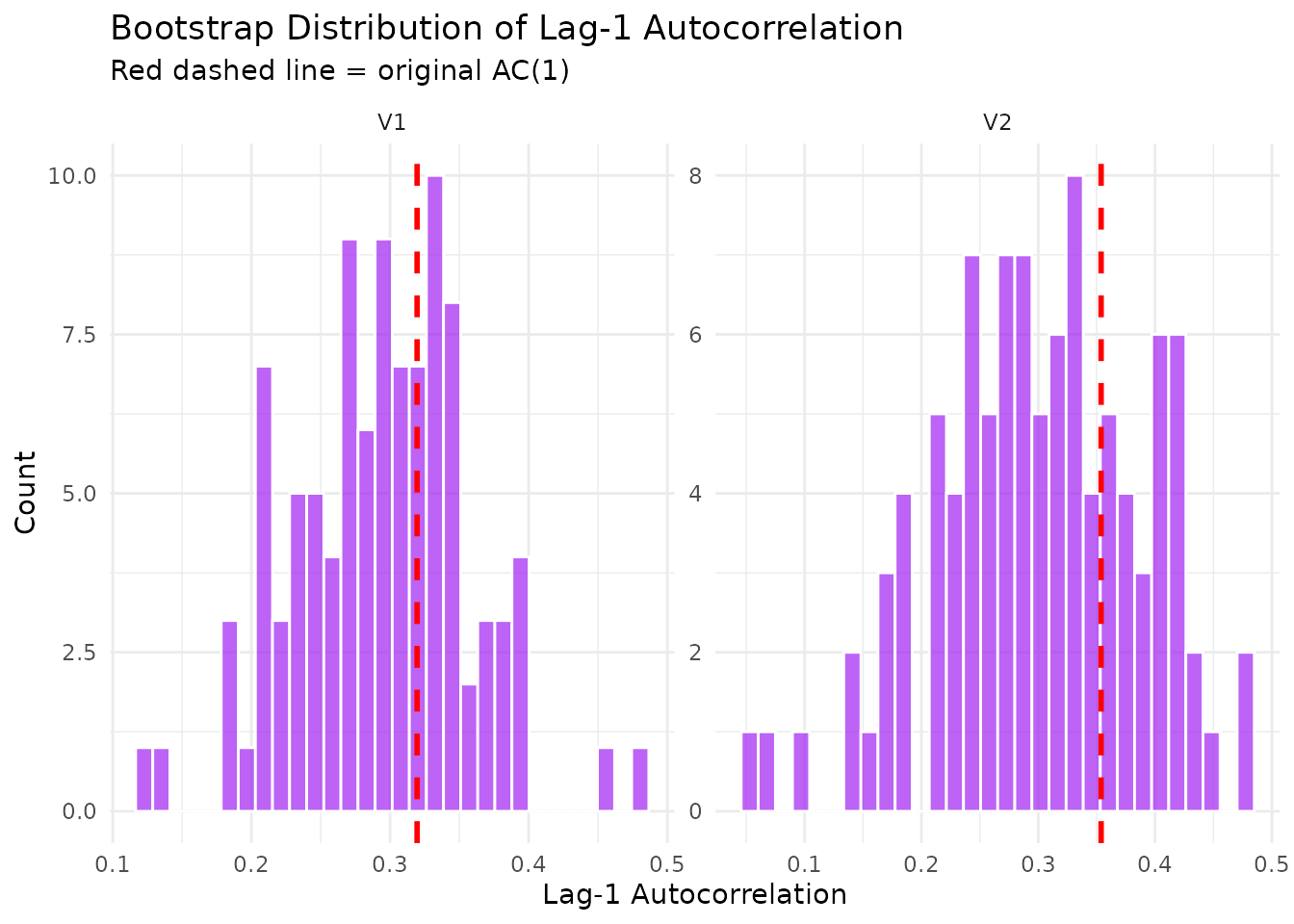

Custom Analysis Examples

The extracted diagnostic data enables custom analyses beyond the built-in summaries.

Bootstrap Confidence Intervals

# Extract bootstrap means
stats_df <- as.data.frame(result$diagnostics, what = "stats")

# Compute percentile confidence interval
ci_95 <- quantile(stats_df$mean_V1, probs = c(0.025, 0.975))
cat("95% Bootstrap CI for mean:", round(ci_95, 4), "\n")
#> 95% Bootstrap CI for mean: -0.3348 0.1195

# Compare to original
cat("Original mean:", round(result$diagnostics$original_stats$means, 4), "\n")
#> Original mean: -0.1558

Assessing Autocorrelation Preservation

# How well does the bootstrap preserve autocorrelation?
orig_ac1 <- result$diagnostics$original_stats$ac1
boot_ac1 <- do.call(rbind, result$diagnostics$series_stats$replicate_ac1)

# Bias in autocorrelation
ac1_bias <- mean(boot_ac1, na.rm = TRUE) - orig_ac1
cat("Original AC(1):", round(orig_ac1, 4), "\n")
#> Original AC(1): 0.6094
cat("Bootstrap AC(1) mean:", round(mean(boot_ac1, na.rm = TRUE), 4), "\n
")
#> Bootstrap AC(1) mean: 0.5377
cat("AC(1) bias:", round(ac1_bias, 4), "\n")
#> AC(1) bias: -0.0717

# What fraction of bootstrap replicates have AC(1) within 0.1 of original?
within_tolerance <- mean(abs(boot_ac1 - orig_ac1) < 0.1, na.rm = TRUE)
cat("Fraction within ±0.1 of original:", round(within_tolerance, 3), "\n")
#> Fraction within ±0.1 of original: 0.73

Block Coverage Analysis

# Analyze how well the bootstrap covers the original series
blocks_df <- extract_blocks(result$diagnostics)

# Distribution of starting positions
start_positions <- blocks_df$start_pos

# Divide original series into deciles and count block starts
n_orig <- result$diagnostics$meta$n_original
decile_breaks <- seq(1, n_orig, length.out = 11)
decile_counts <- hist(start_positions, breaks = decile_breaks, plot = FALSE)$counts

# Check for uniform coverage (chi-square test)
expected <- length(start_positions) / 10
chi_sq <- sum((decile_counts - expected)^2 / expected)
p_value <- pchisq(chi_sq, df = 9, lower.tail = FALSE)

cat("Chi-square test for uniform block coverage:\n")
#> Chi-square test for uniform block coverage:
cat("  Chi-square statistic:", round(chi_sq, 2), "\n")
#>   Chi-square statistic: 30.81
cat("  p-value:", round(p_value, 4), "\n")
#>   p-value: 3e-04
cat("  Interpretation:", ifelse(p_value > 0.05, 
                                 "Coverage appears uniform", 
                                 "Coverage may be non-uniform"), "\n")
#>   Interpretation: Coverage may be non-uniform

Comparing Bootstrap Methods

# Compare moving vs stationary bootstrap
set.seed(999)
x_compare <- as.matrix(arima.sim(n = 200, list(ar = 0.8)))

result_moving <- tsbs(
  x = x_compare,
  block_length = 10,
  bs_type = "moving",
  n_boot = 200,
  num_boots = 200,
  return_diagnostics = TRUE
)

result_stationary <- tsbs(
  x = x_compare,
  bs_type = "stationary",
  block_length = 10,  # Expected block length
  n_boot = 200,
  num_boots = 200,
  return_diagnostics = TRUE
)

# Compare AC(1) preservation
ac1_orig <- acf(x_compare, lag.max = 1, plot = FALSE)$acf[2, 1, 1]

ac1_moving <- do.call(rbind, result_moving$diagnostics$series_stats$replicate_ac1)
ac1_stationary <- do.call(rbind, result_stationary$diagnostics$series_stats$replicate_ac1)

comparison <- data.frame(
  Method = c("Original", "Moving Block", "Stationary"),
  `AC(1) Mean` = c(ac1_orig, mean(ac1_moving), mean(ac1_stationary)),
  `AC(1) SD` = c(NA, sd(ac1_moving), sd(ac1_stationary)),
  check.names = FALSE
)

knitr::kable(comparison, digits = 4, 
             caption = "Autocorrelation Preservation by Bootstrap Method")

Autocorrelation Preservation by Bootstrap Method
Method	AC(1) Mean	AC(1) SD
Original	0.7576	NA
Moving Block	0.6862	0.0488
Stationary	0.6479	0.0607

Best Practices

Choosing Block Length

The block length is a critical parameter for block bootstrap methods. Use diagnostics to assess your choice:

# Try different block lengths and compare AC(1) preservation
block_lengths <- c(5, 10, 15, 20, 25)
ac1_results <- sapply(block_lengths, function(bl) {
  res <- tsbs(x = x_ar, block_length = bl, bs_type = "moving",
              n_boot = 200, num_boots = 100, return_diagnostics = TRUE)
  boot_ac1 <- do.call(rbind, res$diagnostics$series_stats$replicate_ac1)
  c(mean = mean(boot_ac1), bias = mean(boot_ac1) - res$diagnostics$original_stats$ac1)
})

Assessing Bootstrap Quality

Key indicators of bootstrap quality:

Low bias: Bootstrap means close to original
Good AC preservation: Bootstrap autocorrelation close to original
Uniform coverage: Blocks sampled evenly across original series
Appropriate variability: Bootstrap SD reflects sampling uncertainty

Number of Replicates

More replicates provide more stable estimates but increase computation time. Use diagnostics to assess convergence:

# Check if bootstrap mean has stabilized
stats_df <- as.data.frame(result$diagnostics, what = "stats")
running_mean <- cumsum(stats_df$mean_V1) / seq_along(stats_df$mean_V1)
plot(running_mean, type = "l", xlab = "Replicate", ylab = "Running Mean",
     main = "Bootstrap Mean Convergence")

Summary

The tsbs diagnostics system provides comprehensive tools for understanding and validating bootstrap analyses:

Function	Purpose
`summary()`	Comprehensive text report
`plot()`	Diagnostic visualizations
`extract_blocks()`	Block composition data
`extract_summary_stats()`	Statistical summaries
`as.data.frame()`	Convert to data frame for custom analysis

By examining these diagnostics, you can:

Verify bootstrap configuration
Assess how well temporal dependence is preserved
Identify potential issues with block selection
Compare different bootstrap methods
Build confidence in your bootstrap inference

Session Info

sessionInfo()
#> R version 4.5.2 (2025-10-31)
#> Platform: x86_64-pc-linux-gnu
#> Running under: Ubuntu 24.04.3 LTS
#> 
#> Matrix products: default
#> BLAS:   /usr/lib/x86_64-linux-gnu/openblas-pthread/libblas.so.3 
#> LAPACK: /usr/lib/x86_64-linux-gnu/openblas-pthread/libopenblasp-r0.3.26.so;  LAPACK version 3.12.0
#> 
#> locale:
#>  [1] LC_CTYPE=C.UTF-8       LC_NUMERIC=C           LC_TIME=C.UTF-8       
#>  [4] LC_COLLATE=C.UTF-8     LC_MONETARY=C.UTF-8    LC_MESSAGES=C.UTF-8   
#>  [7] LC_PAPER=C.UTF-8       LC_NAME=C              LC_ADDRESS=C          
#> [10] LC_TELEPHONE=C         LC_MEASUREMENT=C.UTF-8 LC_IDENTIFICATION=C   
#> 
#> time zone: UTC
#> tzcode source: system (glibc)
#> 
#> attached base packages:
#> [1] stats     graphics  grDevices utils     datasets  methods   base     
#> 
#> other attached packages:
#> [1] tsbs_0.1.0
#> 
#> loaded via a namespace (and not attached):
#>   [1] tidyselect_1.2.1            dplyr_1.1.4                
#>   [3] farver_2.1.2                S7_0.2.1                   
#>   [5] fastmap_1.2.0               tsgarch_1.0.3              
#>   [7] JADE_2.0-4                  fontquiver_0.2.1           
#>   [9] GeneralizedHyperbolic_0.8-7 digest_0.6.39              
#>  [11] timechange_0.4.0            lifecycle_1.0.5            
#>  [13] cluster_2.1.8.1             tsmarch_1.0.0              
#>  [15] Rsolnp_2.0.1                mev_2.1                    
#>  [17] magrittr_2.0.4              compiler_4.5.2             
#>  [19] rlang_1.1.7                 sass_0.4.10                
#>  [21] tools_4.5.2                 yaml_2.3.12                
#>  [23] data.table_1.18.2.1         knitr_1.51                 
#>  [25] labeling_0.4.3              askpass_1.2.1              
#>  [27] curl_7.0.0                  alabama_2025.1.0           
#>  [29] xml2_1.5.2                  TTR_0.24.4                 
#>  [31] RColorBrewer_1.1-3          abind_1.4-8                
#>  [33] KernSmooth_2.23-26          withr_3.0.2                
#>  [35] nleqslv_3.3.5               purrr_1.2.1                
#>  [37] numDeriv_2016.8-1.1         desc_1.4.3                 
#>  [39] grid_4.5.2                  gdtools_0.4.4              
#>  [41] xts_0.14.1                  future_1.69.0              
#>  [43] progressr_0.18.0            ggplot2_4.0.1              
#>  [45] iterators_1.0.14            globals_0.18.0             
#>  [47] scales_1.4.0                MASS_7.3-65                
#>  [49] cli_3.6.5                   rmarkdown_2.30             
#>  [51] ragg_1.5.0                  generics_0.1.4             
#>  [53] RcppParallel_5.1.11-1       RcppBessel_1.0.0           
#>  [55] future.apply_1.20.1         cachem_1.1.0               
#>  [57] parallel_4.5.2              vctrs_0.7.1                
#>  [59] Matrix_1.7-4                sandwich_3.1-1             
#>  [61] jsonlite_2.0.0              fontBitstreamVera_0.1.1    
#>  [63] clue_0.3-66                 listenv_0.10.0             
#>  [65] systemfonts_1.3.1           foreach_1.5.2              
#>  [67] tidyr_1.3.2                 jquerylib_0.1.4            
#>  [69] quantmod_0.4.28             glue_1.8.0                 
#>  [71] parallelly_1.46.1           pkgdown_2.2.0              
#>  [73] nloptr_2.2.1                SkewHyperbolic_0.4-2       
#>  [75] codetools_0.2-20            DistributionUtils_0.6-2    
#>  [77] shape_1.4.6.1               lubridate_1.9.4            
#>  [79] flextable_0.9.10            gtable_0.3.6               
#>  [81] tsmethods_1.0.2             tibble_3.3.1               
#>  [83] pillar_1.11.1               htmltools_0.5.9            
#>  [85] openssl_2.3.4               truncnorm_1.0-9            
#>  [87] R6_2.6.1                    TMB_1.9.19                 
#>  [89] textshaping_1.0.4           Rdpack_2.6.5               
#>  [91] evaluate_1.0.5              lattice_0.22-7             
#>  [93] rbibutils_2.4.1             fontLiberation_0.1.0       
#>  [95] bslib_0.10.0                Rcpp_1.1.1                 
#>  [97] zip_2.3.3                   uuid_1.2-2                 
#>  [99] officer_0.7.3               xfun_0.56                  
#> [101] fs_1.6.6                    zoo_1.8-15                 
#> [103] pkgconfig_2.0.3             tsdistributions_1.0.3

Understanding and Analyzing Bootstrap Output in tsbs

tsbs Package

2026-01-31