Hidden Markov Model (HMM) Bootstrap for Multivariate Time Series

Fits a Gaussian Hidden Markov Model (HMM) to a multivariate time series and generates bootstrap replicates by resampling regime-specific blocks.

Usage

hmm_bootstrap_old(
  x,
  n_boot = NULL,
  num_states = 2,
  num_blocks = NULL,
  num_boots = 100,
  parallel = FALSE,
  num_cores = 1L,
  return_fit = FALSE,
  collect_diagnostics = FALSE,
  verbose = FALSE
)

Arguments

x

Numeric vector or matrix representing the time series.

n_boot

Length of bootstrap series.

num_states

Integer number of hidden states for the HMM.

num_blocks

Integer number of blocks to sample for each bootstrap replicate.

num_boots

Integer number of bootstrap replicates to generate.

parallel

Parallelize computation? TRUE or FALSE.

num_cores

Number of cores.

return_fit

Logical. If TRUE, returns the fitted HMM model along with bootstrap samples. Default is FALSE.

collect_diagnostics

Logical. If TRUE, collects detailed diagnostic information including regime composition of each bootstrap replicate. Default is FALSE.

verbose

Logical. If TRUE, prints HMM fitting information and warnings. Defaults to FALSE.

Value

If return_fit = FALSE and collect_diagnostics = FALSE: A list of bootstrap replicate matrices.

If return_fit = TRUE or collect_diagnostics = TRUE: A list containing:

bootstrap_series

List of bootstrap replicate matrices

fit

(if return_fit = TRUE) The fitted depmixS4 model object

states

The Viterbi state sequence for the original data

diagnostics

(if collect_diagnostics = TRUE) A tsbs_diagnostics object

Details

This function:

• Fits a Gaussian HMM to x using depmixS4::depmix() and depmixS4::fit().

• Uses Viterbi decoding (posterior(fit, type = "viterbi")$state) to assign each observation to a state.

• Samples contiguous blocks of observations belonging to each state.

If n_boot is set, the last block will be trimmed when necessary. If n_boot is not set, and num_blocks is set, the length of each bootstrap series will be determined by the number of blocks and the random lengths of the individual blocks for that particular series. If neither n_boot nor num_blocks is set, n_boot will default to the number of rows in x and the last block will be trimmed when necessary.

For multivariate series (matrices or data frames), the function fits a single HMM where all variables are assumed to depend on the same underlying hidden state sequence. The returned bootstrap samples are matrices with the same number of columns as the input x.

Hidden Markov Model definition:

• \(T\): sequence length

• \(K\): number of hidden states

• \(\mathbf{X} = (X_1, \dots, X_T)\): observed sequence

• \(\mathbf{S} = (S_1, \dots, S_T)\): hidden (latent) state sequence

• \(\pi_i = \mathbb{P}(S_1 = i)\): initial state distribution

• \(A = [a_{ij}], \text{ where } a_{ij} = \mathbb{P}(S_{t+1} = j \mid S_t = i)\): transition matrix

• \(b_j(x_t) = \mathbb{P}(X_t = x_t \mid S_t = j)\): output probability

Joint probability of the observations and the hidden states:

\(\mathbb{P}(\mathbf{X}, \mathbf{S}) = \pi_{S_1} b_{S_1}(X_1) \prod_{t=2}^{T} a_{S_{t-1} S_t} b_{S_t}(X_t)\)

Marginal probability of the observed data is obtained by summing over all possible hidden state sequences:

\(\mathbb{P}(\mathbf{X}) = \sum_{\mathbf{S}} \mathbb{P}(\mathbf{X}, \mathbf{S})\)

(Beware of the "double use of data" problem: The bootstrap procedure relies on regime classification, but the regimes themselves are estimated from the same data and depend on the parameters being resampled.)

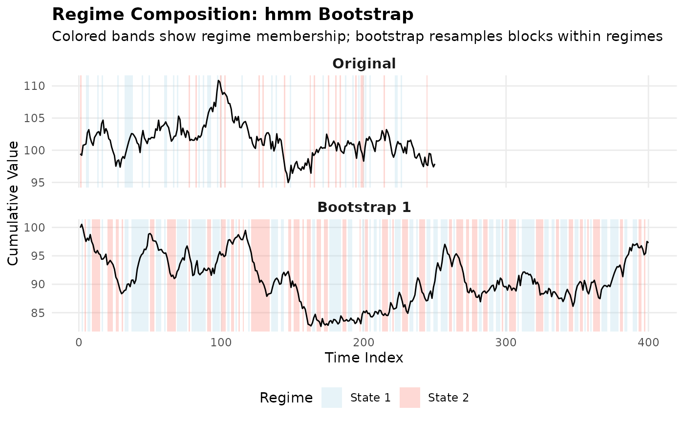
When collect_diagnostics = TRUE, the function records:

• Original state sequence from Viterbi decoding

• State sequence for each bootstrap replicate

• Block information (lengths, source positions)

This information can be used with plot_regime_composition() to visualize how the bootstrap samples are composed from different regimes.

References

Holst, U., Lindgren, G., Holst, J. and Thuvesholmen, M. (1994), Recursive Estimation In Switching Autoregressions With A Markov Regime. Journal of Time Series Analysis, 15: 489-506. https://doi.org/10.1111/j.1467-9892.1994.tb00206.x

Examples

# \donttest{
# Requires depmixS4 package
if (requireNamespace("depmixS4", quietly = TRUE)) {

  ## Example 1: Univariate time series with regime switching
  set.seed(123)
  # Generate data with two regimes
  n1 <- 100
  n2 <- 100
  regime1 <- rnorm(n1, mean = 0, sd = 1)
  regime2 <- rnorm(n2, mean = 5, sd = 2)
  x_univar <- c(regime1, regime2)

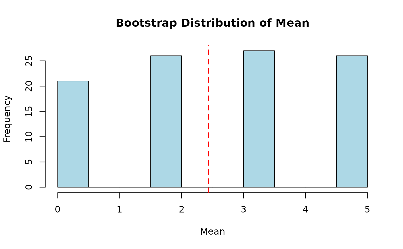
  # Generate bootstrap samples
  boot_samples <- hmm_bootstrap(
    x = x_univar,
    n_boot = 150,
    num_states = 2,
    num_boots = 100
  )

  # Inspect results
  length(boot_samples)  # 100 bootstrap replicates
  dim(boot_samples[[1]])  # Each is a 150 x 1 matrix

  # Compare original and bootstrap distributions
  original_mean <- mean(x_univar)
  boot_means <- sapply(boot_samples, mean)

  hist(boot_means, main = "Bootstrap Distribution of Mean",
       xlab = "Mean", col = "lightblue")
  abline(v = original_mean, col = "red", lwd = 2, lty = 2)


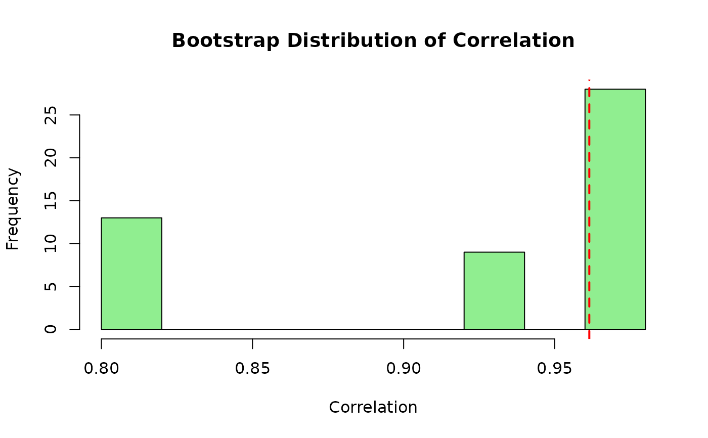
  ## Example 2: Multivariate time series
  set.seed(456)
  n <- 200
  # Two correlated series with regime switching
  states_true <- rep(1:2, each = n/2)
  x1 <- ifelse(states_true == 1,
               rnorm(n, 0, 1),
               rnorm(n, 4, 2))
  x2 <- 0.7 * x1 + rnorm(n, 0, 0.5)
  x_multivar <- cbind(x1, x2)

  boot_samples_mv <- hmm_bootstrap(
    x = x_multivar,
    n_boot = 180,
    num_states = 2,
    num_boots = 50
  )

  dim(boot_samples_mv[[1]])  # 180 x 2 matrix

  # Compute bootstrap correlation estimates
  boot_cors <- sapply(boot_samples_mv, function(b) cor(b[,1], b[,2]))
  original_cor <- cor(x_multivar[,1], x_multivar[,2])

  hist(boot_cors, main = "Bootstrap Distribution of Correlation",
       xlab = "Correlation", col = "lightgreen")
  abline(v = original_cor, col = "red", lwd = 2, lty = 2)


  ## Example 3: Variable-length bootstrap samples
  set.seed(789)
  x_ar <- arima.sim(n = 150, list(ar = 0.8))

  # Don't specify n_boot to get variable-length samples
  boot_samples_var <- hmm_bootstrap(
    x = x_ar,
    n_boot = NULL,  # Variable length
    num_states = 2,
    num_blocks = 15,
    num_boots = 20
  )

  # Check lengths vary
  sample_lengths <- sapply(boot_samples_var, nrow)
  summary(sample_lengths)


  ## Example 4: Using verbose mode for diagnostics
  set.seed(321)
  x_diag <- rnorm(100)

  boot_samples_verbose <- hmm_bootstrap(
    x = x_diag,
    n_boot = 80,
    num_states = 3,
    num_boots = 5,
    verbose = TRUE  # Print diagnostic information
  )


  ## Example 5: Bootstrap confidence intervals
  set.seed(654)
  # Data with heteroskedasticity
  n <- 200
  x_hetero <- numeric(n)
  for (i in 1:n) {
    sigma <- ifelse(i <= n/2, 1, 3)
    x_hetero[i] <- rnorm(1, mean = 2, sd = sigma)
  }

  boot_samples_ci <- hmm_bootstrap(
    x = x_hetero,
    n_boot = 200,
    num_states = 2,
    num_boots = 500
  )

  # Compute bootstrap confidence interval for the mean
  boot_means_ci <- sapply(boot_samples_ci, mean)
  ci_95 <- quantile(boot_means_ci, c(0.025, 0.975))

  cat("95% Bootstrap CI for mean:", ci_95[1], "to", ci_95[2], "\n")
  cat("Original mean:", mean(x_hetero), "\n")


  ## Example 6: Basic usage
  set.seed(123)
  x <- matrix(rnorm(500), ncol = 2)
  boot_samples <- hmm_bootstrap(x, n_boot = 400, num_states = 2, num_boots = 50)

  ## With diagnostics for regime visualization
  result <- hmm_bootstrap(
    x, n_boot = 400, num_states = 2, num_boots = 10,
    collect_diagnostics = TRUE, return_fit = TRUE
  )

  ## Plot regime composition
  plot_regime_composition(result, x)
}
#> converged at iteration 14 with logLik: -345.2058 

#> converged at iteration 21 with logLik: -641.5917 

#> converged at iteration 22 with logLik: -237.4892 
#> Fitting 3-state Gaussian HMM to 1-dimensional series of length 100...
#> iteration 0 logLik: -136.5052 
#> iteration 5 logLik: -136.1879 
#> iteration 10 logLik: -136.0729 
#> iteration 15 logLik: -135.9875 
#> iteration 20 logLik: -135.7953 
#> iteration 25 logLik: -135.2338 
#> iteration 30 logLik: -133.9723 
#> iteration 35 logLik: -131.707 
#> iteration 40 logLik: -128.8447 
#> iteration 45 logLik: -127.3979 
#> iteration 50 logLik: -126.9794 
#> iteration 55 logLik: -126.8497 
#> iteration 60 logLik: -126.806 
#> iteration 65 logLik: -126.7847 
#> iteration 70 logLik: -126.7683 
#> iteration 75 logLik: -126.7525 
#> iteration 80 logLik: -126.7373 
#> iteration 85 logLik: -126.7237 
#> iteration 90 logLik: -126.7126 
#> iteration 95 logLik: -126.7041 
#> iteration 100 logLik: -126.6979 
#> iteration 105 logLik: -126.6934 
#> iteration 110 logLik: -126.69 
#> iteration 115 logLik: -126.6874 
#> iteration 120 logLik: -126.6854 
#> iteration 125 logLik: -126.6839 
#> iteration 130 logLik: -126.6826 
#> iteration 135 logLik: -126.6816 
#> iteration 140 logLik: -126.6808 
#> iteration 145 logLik: -126.6801 
#> iteration 150 logLik: -126.6796 
#> iteration 155 logLik: -126.6791 
#> iteration 160 logLik: -126.6787 
#> iteration 165 logLik: -126.6784 
#> iteration 170 logLik: -126.6781 
#> iteration 175 logLik: -126.6779 
#> iteration 180 logLik: -126.6777 
#> iteration 185 logLik: -126.6776 
#> iteration 190 logLik: -126.6774 
#> iteration 195 logLik: -126.6773 
#> iteration 200 logLik: -126.6772 
#> iteration 205 logLik: -126.6772 
#> iteration 210 logLik: -126.6771 
#> iteration 215 logLik: -126.677 
#> iteration 220 logLik: -126.677 
#> iteration 225 logLik: -126.6769 
#> iteration 230 logLik: -126.6769 
#> iteration 235 logLik: -126.6769 
#> iteration 240 logLik: -126.6769 
#> iteration 245 logLik: -126.6768 
#> iteration 250 logLik: -126.6768 
#> iteration 255 logLik: -126.6768 
#> iteration 260 logLik: -126.6768 
#> iteration 265 logLik: -126.6768 
#> iteration 270 logLik: -126.6768 
#> iteration 275 logLik: -126.6768 
#> converged at iteration 280 with logLik: -126.6768 
#> State distribution: 1 = 19, 2 = 47, 3 = 34
#> Generating 5 bootstrap samples...
#> Bootstrap complete. Generated 5 samples.
#> converged at iteration 22 with logLik: -393.5627 
#> 95% Bootstrap CI for mean: 1.60645 to 1.878304 
#> Original mean: 1.747322 
#> converged at iteration 184 with logLik: -687.2476 
#> converged at iteration 175 with logLik: -687.2476 

# }